Introduction
Buy a sensor, open the datasheet, and somewhere on the first page you will find one of these:
“Interface: I2C” “Interface: SPI” “Interface: UART”
And the first question is always the same:
"…so what is the difference, and which one do I want?"
Go one step past blinking an LED and try to attach a sensor, and you hit this wall immediately. Temperature and humidity sensors are I2C, SD cards are SPI, GPS modules are UART. All three are called “serial communication”, yet the wiring and the library calls are completely different.
This article puts the three side by side on the same terms. It is not an implementation guide for any one of them — it is about the criteria for deciding which one to use.
📝 What you will learn:
- The structural differences between I2C, SPI and UART (why the wire counts differ)
- The three axes that decide the choice: speed, device count, and distance
- How to tell, before you buy a part, whether it will work in your setup
- What to look for when you put a communication bus on an oscilloscope
Written for readers who have got as far as blinking an LED on an Arduino and reading a sensor value in the Serial Monitor. The microcontroller does not matter — Arduino, ESP32 or STM32, the reasoning behind these three buses is the same.
🔍 The Three Protocols at a Glance
Before the details, here is the conclusion. If you take away only this table, you have 90% of it.
| UART | I2C | SPI | |
|---|---|---|---|
| Signal lines | 2 (TX / RX) | 2 (SDA / SCL) | 4 (SCK / MOSI / MISO / CS) |
| Clock line | none (asynchronous) | yes (SCL) | yes (SCK) |
| Typical speed | 9,600–115,200 bps | 100k / 400k bps (up to 1M–3.4M in fast modes) | a few MHz to tens of MHz |
| Master / slave | peers (point to point) | master / slave (multi-master possible) | master / slave |
| Multiple devices | ❌ one to one, essentially | ⭕ around 100 devices, by address | △ one more CS line per device |
| Practical distance | a few metres (TTL levels) | around 1 m (really an on-board bus) | tens of cm (on-board) |
| Duplex | full duplex | half duplex | full duplex |
| Acknowledgement (ACK) | none | yes (per byte) | none |
| Pull-up resistors | not needed | mandatory | not needed |
| Best suited to | GPS, radio modules, debug link to a PC | temperature/humidity and pressure sensors, GPIO expander ICs, EEPROM | SD cards, TFT displays, fast ADCs, shift registers |
In three lines
- Need fewer wires, or want to hang a lot of sensors off one bus → I2C
- Need raw speed, or are moving a lot of data → SPI
- Talking to a single “module”, and want some distance → UART
The rest of the article explains why each row of that table comes out the way it does.
📡 UART — Agreeing on a Speed and Nothing Else
UART (Universal Asynchronous Receiver/Transmitter) is the simplest of the three, and by far the oldest.
The defining feature: there is no clock line
UART has no clock line. That is the decisive difference from I2C and SPI.
With I2C or SPI, the transmitter tells you “read a bit now” over a dedicated clock wire. UART has nothing of the sort. So how do the two ends stay in step?
The answer is that they agree on a speed in advance. That agreement is the baud rate.
Serial.begin(9600); // "I will speak at 9600 bits per second"
At 9,600 bps, the time occupied by one bit falls out directly:
T_{bit} = \frac{1}{9600} \approx 104.17\ \mu sThe receiver knows that once the start bit arrives, it should sample eight times at 104.17 µs intervals. In other words, time itself is standing in for the clock.
When the Serial Monitor fills up with characters like ��������, nine times out of ten the transmitter and receiver are set to different baud rates. Match the value in Serial.begin() with the setting in the bottom-right corner of the Serial Monitor. Check that before you start suspecting your wiring.
The structure of one frame
UART sends one byte at a time, wrapped in a “frame”. The most common arrangement is 8N1 — 8 data bits, no parity, 1 stop bit:
| Section | Bits | Level | Purpose |
|---|---|---|---|
| Idle | — | H | Nothing being sent |
| Start bit | 1 | L | “Here it comes” |
| Data bits | 8 | varies | Sent LSB first |
| Parity bit | 0 or 1 | varies | Error detection (usually omitted) |
| Stop bit | 1–2 | H | “That’s the end of it” |
The LSB-first ordering matters. Send 0x41 (the character A) and what actually goes down the wire is 1,0,0,0,0,0,1,0. Try to read a waveform without keeping bit order in mind and you will confuse yourself every time.
The one-to-one constraint
UART has no concept of an address. It talks to exactly one partner, wired TX-to-RX and RX-to-TX. It is strictly point to point.
That makes it fundamentally unsuited to hanging three sensors off one bus. It is, on the other hand, ideal for the case where you have a single counterpart — a GPS or Bluetooth module — streaming data back and forth indefinitely.
At raw TTL levels (0 V / 3.3 V or 5 V) a few metres is the practical limit, but drop an RS-232 or RS-485 transceiver in the middle and the reach extends dramatically. That extensibility is exactly why “if you need distance, you want something UART-based” is the standard advice.
🔗 I2C — Any Number of Devices on Two Wires
I2C (Inter-Integrated Circuit) connects multiple devices in a chain over just two wires: SDA (data) and SCL (clock).
Microcontroller pins are a finite resource. If every additional sensor costs you two more of them, you run out fast. I2C solves that by having everyone share the same two wires.
Calling devices by address
If the wires are shared, you need a way to say who you are talking to. That is the slave address, normally 7 bits.
The master opens a transaction with, effectively, “device at address 0x27, answer me”, and only the matching device replies. Seven bits give 128 combinations in theory; once reserved addresses are excluded you get around 112 usable devices.
In practice, though, you hit a different problem: two identical sensors have the same address and collide. Which is why most ICs give you external pins that set the low bits of the address by tying them high or low. The A0/A1/A2 pins covered in the MCP23017 article are exactly this — three pins generate eight distinct addresses, so you can line up eight of the same chip.
Why pull-up resistors are mandatory
The single most common way to get stuck on your first I2C project is forgetting the pull-up resistors. “The wiring is right but a bus scan finds nothing at all” is almost always this.
Why are they required? Because I2C outputs are open-drain.
Every device on the bus can only ever pull the line down to GND. Nobody has the ability to drive it high. That is a necessary consequence of sharing one wire: if devices could drive high freely, the instant one drove high while another drove low you would short the supply straight to ground.
So an external resistor holds the line up at the supply voltage (the pull-up), and whenever nobody is pulling it down, it settles high on its own.
The lower bound comes from the requirement that the current flowing when the line is pulled low must not exceed the IC’s sink capability (IOL, typically 3 mA).
R_{p(min)} = \frac{V_{DD} - V_{OL(max)}}{I_{OL}}With a 3.3 V supply, VOL = 0.4 V and IOL = 3 mA, that puts the floor at roughly 970 Ω.
The upper bound comes from how quickly the bus capacitance can be charged.
R_{p(max)} = \frac{t_r}{0.8473 \times C_b}In standard mode (rise time tr = 1000 ns) with a bus capacitance Cb = 100 pF, the ceiling is about 11.8 kΩ.
In practice, 4.7 kΩ at 100 kHz and 2.2 kΩ at 400 kHz will almost never let you down. If the resistor arithmetic itself is the shaky part, read the Ohm’s law article first.
Note that many sensor breakout boards already have pull-ups fitted. In that case you do not add any. But the opposite problem then appears: connect several such modules in parallel and their pull-ups end up in parallel too, dropping the effective resistance too far. Beyond about three modules you may need to remove the pull-ups from all but one of them.
Start and stop, expressed as line movements
I2C has a convention the other two do not: the start condition and the stop condition.
| Condition | SCL | SDA | Meaning |
|---|---|---|---|
| Start | stays H | falls H → L | Transaction begins |
| Stop | stays H | rises L → H | Transaction ends |
| During data | only while L | may change | Ordinary bit transfer |
Normally SDA only ever changes while SCL is low. “SDA moved while SCL was high” is therefore a rule violation being used deliberately as a signal. That trick is what lets I2C distinguish control events from data without spending an extra wire on it.
ACK — the only one of the three that confirms delivery
After every 8 bits, I2C gives the receiver a 9th clock in which to pull SDA low. That is the ACK (acknowledge).
Of the three protocols, I2C is the only one where the receiver says “got it”. If no device responds, SDA stays high (a NACK) and the master knows immediately that nothing lives at that address.
This is the entire reason an I2C scanner sketch works. It simply calls out to every address in turn and lists the ones that answer with an ACK.
⚡ SPI — The Choice When You Need Speed
SPI (Serial Peripheral Interface) is built around speed above all else. SD cards, TFT displays, fast A/D converters — anything shifting a lot of data is almost certainly on SPI.
What the four wires do
| Signal | Also called | Direction | Role |
|---|---|---|---|
| SCK | SCLK / CLK | master → slave | Clock |
| MOSI | SDO / COPI | master → slave | Data from the master |
| MISO | SDI / CIPO | slave → master | Data from the slave |
| CS | SS / NSS | master → slave | Select this device (usually active low) |
Because the transmit and receive lines are separate, SPI can send and receive at the same time (full duplex). I2C shares a single SDA line for both directions and is therefore half duplex — a structural difference, not a tuning detail.
Why it is fast
SPI is fast largely because of everything it declines to do.
- No addressing (devices are selected physically, with CS)
- No ACK (delivery is never confirmed)
- No start/stop conditions (the transaction begins the moment CS goes low)
- Push-pull outputs rather than open-drain (both H and L are driven actively)
Protocol overhead is essentially zero, and because the outputs actively drive high, SPI does not suffer the edge-rounding that a pull-up resistor working against bus capacitance causes on I2C. Tens of MHz are realistic as a result.
The price is wire count. Every extra device costs another CS line: three devices means SCK, MOSI, MISO and 3× CS, six wires in total. I2C stays at two no matter how many devices you add. Think of it as SPI buying its speed with pins, and the trade-off becomes easy to reason about.
Modes 0–3 — the classic SPI trap
There is one thing SPI deliberately does not pin down: which clock edge the data is sampled on. The combination of CPOL (clock polarity) and CPHA (clock phase) gives four possibilities.
| Mode | CPOL | CPHA | SCK when idle | Data sampled on |
|---|---|---|---|---|
| 0 | 0 | 0 | L | rising edge |
| 1 | 0 | 1 | L | falling edge |
| 2 | 1 | 0 | H | falling edge |
| 3 | 1 | 1 | H | rising edge |
Mode 0 is by far the most common, but some devices insist on mode 3.
If an SPI device returns all 0x00, all 0xFF, or values that look like the real thing shifted by one bit, a mode mismatch is the first suspect. Check the timing diagram in the datasheet for the idle level of SCK and the point at which data is valid.
Unlike I2C, SPI has no ACK, so nothing tells you the transfer failed. You just quietly get corrupted data back. That is a property to keep in mind the whole time you are working with SPI.
SPI seen from the register level
From the microcontroller’s point of view, SPI is little more than “clock a shift register eight times”. Driving a 74HC595 shift register with shiftOut() and sending a byte over SPI are, at the hardware level, very nearly the same operation.
If you already understand the 74HC595, SPI clicks into place as “the version where the hardware does that for you”.
To go a level deeper into what happens in the registers, Episode 4 of the STM32 series (the world of bits — register operations) is a good next stop. And when you are streaming large amounts of pixel data to a display over SPI, pairing it with the DMA covered in Episode 10 is the standard approach.
📊 Making Sense of the Waveforms
For some of the differences between these three, one look at the shape of the signals beats any amount of prose.
What follows are timing diagrams — idealized drawings of how each protocol’s signals line up. On real hardware you get rounded edges and noise on top of this, but a clean diagram is easier to learn “where to look” from. So the intended order is: get the structure from the diagram first, then compare it against the real thing on your own scope.
Settings for measuring it yourself
These are the scope settings for seeing, on real hardware, what the diagrams show.
| Item | Setting |
|---|---|
| Channels | 2 (one for the clock, one for the data) |
| Probe | ×10 (×1 lacks the bandwidth and rounds the edges) |
| Ground | Always clip the probe ground to the ground of the circuit under test |
| Trigger | Falling edge, single shot |
Single shot matters. Communication happens in bursts rather than continuously, so a free-running display just smears the waveform past you.
UART: sending 0x55
UART needs only one probe, which makes it the easiest place to start. For test data, 0x55 (the character U) is the one to use.
0x55 is 0101 0101 in binary. Sent LSB first, the line carries 1,0,1,0,1,0,1,0 — a clean square wave. The bit boundaries are countable by eye, which is exactly what you want the first time you look at a serial waveform.
void setup() {
  Serial.begin(9600);
}

void loop() {
  Serial.write(0x55);   // fixed pattern for observation
  delay(100);
}
Three things to read off:
- Is the idle level high? — if it sits low, you are on the wrong pin for TX
- The width of one bit — about 104 µs at 9,600 bps. If that is off, the baud rate setting is wrong
- Where the start bit (the first L) is — that is your reference point for counting bits
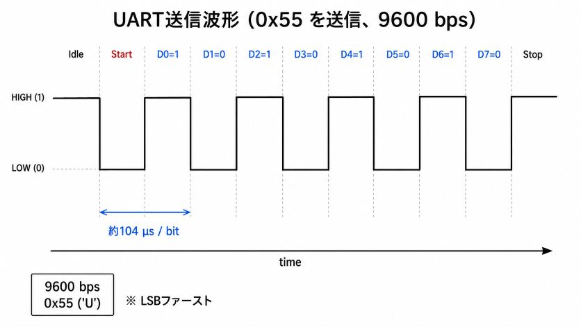
Timing diagram: one UART frame carrying 0x55 at 9,600 bps. From the falling edge of the start bit, the bits line up at roughly 104 µs intervals
When you do not know what baud rate a module is using, measure the width of one bit and invert it.
\text{baud} = \frac{1}{T_{bit}}8.68 µs per bit means 115,200 bps; 104 µs means 9,600 bps. Worth remembering as a practical technique for reverse-engineering a module of unknown baud rate.
I2C: watching SCL and SDA together
I2C uses both channels. Put SCL on CH1 and SDA on CH2, and trigger on the falling edge of SDA.
Three things to look for:
- The start condition — the moment SDA falls while SCL is still high. That is the origin of the transaction
- The 7 address bits — the first seven clocks. Read those and you know which device is being addressed
- The ACK on the 9th clock — SDA pulled low means the device answered; SDA still high is a NACK
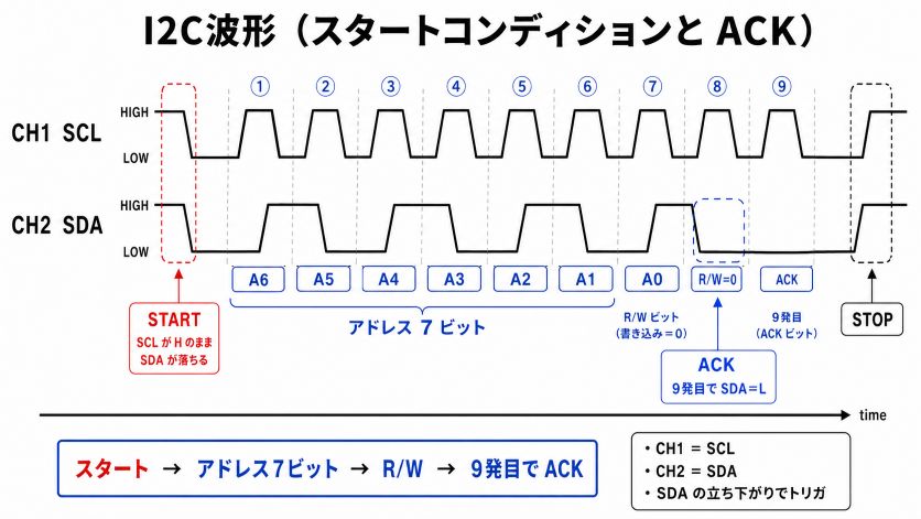
Timing diagram: one I2C transaction. SDA falls while SCL is high (start) → 7 address bits → SDA is pulled low on the 9th clock (ACK)
Where real hardware differs from the diagram
In the diagram above the signals rise vertically. On a real I2C bus, this is precisely where the edges round off the most.
An open-drain output can only pull low, so the return to high depends on the pull-up resistor charging the bus capacitance. Real SDA and SCL lines therefore have sloped rising edges. If the slope is severe enough that the signal looks triangular, your pull-up is too large — the receiver can no longer reliably read a high as a high, and the bus becomes unstable. Going one step down (4.7 kΩ → 2.2 kΩ) usually fixes it.
None of that rounding is drawn in the diagram; you only see it once you measure real hardware. An unstable I2C bus is the single clearest case for owning an oscilloscope.
SPI: two channels are not enough for CS
SPI has four signals, so a two-channel scope cannot show you the whole picture at once. There is no way around that; you have to pick.
In practice there are two useful pairings:
| What you want to see | CH1 | CH2 |
|---|---|---|
| The mode (recommended) | SCK | MOSI |
| CS timing | CS | SCK |
Start with SCK + MOSI to establish the mode — the idle level of SCK, and the edge on which data is valid. Ideally you would trigger on the falling edge of CS, but with only two channels, triggering on the first SCK edge is a workable substitute.
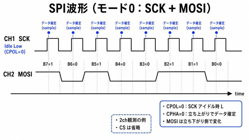
Timing diagram: SCK and MOSI in SPI mode 0. SCK idles low, and data is valid on the rising edge
On real hardware, here is what to read:
- SCK idle low means CPOL = 0; idle high means CPOL = 1
- Where MOSI changes relative to the SCK edges → this tells you CPHA
- SPI uses push-pull outputs, so the corners stay sharp even on real hardware. If they are rounded, your wiring is too long
If you measure I2C and SPI under the same conditions and put them side by side, the contrast is obvious: I2C’s rising edges lean over, SPI’s corners stand up. It is the clearest demonstration there is of the difference between open-drain and push-pull.
🧭 So Which One Should You Use?
Work through it in this order and the decision stops being difficult.
Step 1: check whether you even have a choice
Most of the time you do not. If the sensor you want only speaks I2C, you are using I2C. Look at the datasheet first.
A real choice only shows up in cases like these:
- The same function is sold in both an I2C and an SPI variant
- You are designing the circuit yourself and get to pick the IC
- You are choosing a display module that supports both
Step 2: answer four questions
| Question | If yes |
|---|---|
| Is there only one device, and is it more than 1 m away? | UART |
| Do you want three or more devices on the same bus? | I2C |
| Are you moving tens of KB per second or more (images, audio, SD card)? | SPI |
| Do you have only two spare pins on the microcontroller? | I2C |
Step 3: when in doubt, start with I2C
If none of the above applies, pick I2C. Three reasons:
- Two wires means fewer opportunities to miswire something on a breadboard
- The ACK tells you immediately when nothing is connected (SPI silently hands back garbage)
- An I2C scanner confirms in a few lines of code whether the device is being seen at all
If it turns out you need more throughput, moving to SPI at that point is easy. There is rarely a good reason to start there. Ease of debugging translates directly into development speed.
On this site, an ESP32 network clock expands its GPIO to 16 pins by hanging an MCP23017 on the I2C bus. The reasoning is straightforward: the display updates about once a second, so speed is simply not a requirement.
Contrast that with multiplexing a high-voltage nixie tube display, or pushing image data into a TFT LCD. There the volume of data is orders of magnitude higher and SPI becomes mandatory.
Estimate up front whether speed matters — in practice that single question decides the protocol.
🛠️ Troubleshooting
| Symptom | Bus | Likely cause | Fix |
|---|---|---|---|
| No devices found at all | I2C | No pull-up resistors | Add 4.7 kΩ on both SDA and SCL |
| Device is found but the data is corrupt | I2C | Pull-up too large, edges rounded | Drop to 2.2 kΩ / shorten the wiring |
| Adding a second device broke both | I2C | Address collision | Change the address with the A0–A2 pins |
| Every read is 0x00 or 0xFF | SPI | Mode mismatch, or CS is not moving | Check CPOL/CPHA in the datasheet |
| Values are off by one bit | SPI | Wrong CPHA | Swap between mode 0 and mode 3 |
| Garbled characters | UART | Baud rate mismatch | Match the setting on both ends |
| Nothing is received at all | UART | TX and RX are not crossed | Wire TX → RX and RX → TX |
| Works, but corrupts occasionally | any | Supply noise, wiring too long | Add decoupling, shorten wiring, slow the bus down |
The ESP32 and STM32 are 3.3 V parts; the Arduino UNO is 5 V. Feeding a 5 V signal straight into a 3.3 V sensor can destroy it.
With I2C you can sometimes solve this simply by pulling up to 3.3 V, but if you want certainty, put a level shifter in the path. The same applies to SPI and UART. “It worked, and then the sensor died a while later” is the classic outcome of skipping this.
✅ Summary
- UART has no clock line and stays in sync purely by agreeing on a baud rate — a “contract about time”. Point to point only, but the easiest to extend over distance
- I2C shares two wires among all devices and picks between them by address. Open-drain outputs make pull-up resistors mandatory. It is the only one of the three with an ACK
- SPI gives up both addressing and acknowledgement, and in exchange is dramatically faster. Each extra device costs a CS line. Mode 0–3 mismatches are the classic pitfall
- The choice comes down to three questions: how much speed, how many devices, and how far
- When in doubt, start with I2C. Having an ACK makes debugging far less painful
Understand these differences structurally and a datasheet for a part you have never used before will tell you, at a glance, how to wire it and what to watch out for. That is the dividing line between blinking an LED and designing your own circuits.
Frequently Asked Questions
Q. A sensor supports both I2C and SPI. Which should I use?
A. If you do not need the speed, use I2C. Two wires, and the ACK makes it easy to confirm the device is connected. Choose SPI only when the data volume is high — screen updates, data logging and the like.
Q. If a module already has pull-up resistors, do I need to add my own?
A. Not for a single module. But connecting several modules in parallel puts their pull-ups in parallel too, dropping the combined resistance too far. With three or more, consider removing the pull-ups from all but one of them.
Q. Can I connect three modules over UART?
A. Not with standard UART. You can connect as many as your microcontroller has UART peripherals (the ESP32 has three; STM32 parts vary, often more). If that is still not enough, it is a strong sign that I2C is the right fit for your design.
Q. What do I do when I cannot work out the SPI mode?
A. The proper method is to read the timing diagram in the datasheet: the idle level of SCK (low means CPOL = 0) and the edge at which data is valid. If the datasheet does not say, try mode 0 and mode 3 — between them they cover the large majority of devices.
Q. Can I debug these buses without an oscilloscope?
A. Up to a point, yes. An I2C scanner sketch tells you whether a device is present, and for UART the Serial Monitor shows you what is arriving. But physical-layer problems — rounded edges, corruption that only appears at higher speeds — cannot be diagnosed without seeing the waveform. That is the boundary where a measuring instrument becomes necessary.
Related Articles
I2C in practice:
SPI and shift registers:
UART and serial basics:
Understanding communication from inside the microcontroller:
- STM32 #4: The World of Bits — Register Operations and the BSRR Design
- STM32 #8: Interrupts — EXTI and NVIC Complete Guide
- STM32 #10: DMA — the Architecture That Keeps the CPU Idle
Putting these signals on a board:
- ESP32 Network Clock (1): PCB Design with KiCad and JLCPCB
- KiCad 10.0 New Features: Importers, Variants, Graphical DRC